gf_point(CorneoDiff ~ Time | Product, data=hyd.sm) |>
gf_lims(x=c(0,24)) 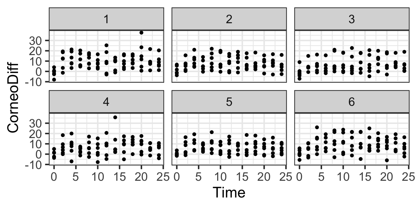
So far, we looked at random effects as one way to account for non-independence of residuals due to a variable that we don’t want to include as a regular predictor. Another option for this kind of situation is to use Generalized Estimating Equations (GEEs).
The dataset used here is industry data from a skin care company. It contains data from experiments with 20 subjects. Each person tested 6 different skin moisturizers, and the hydration level of their skin was measured every 2 hours for 24 hours following application of each product. The variables are:
Subjects Numeric code identifying the personCorneoDiff The hydration CorneoDiffTime Time in hours since product applicationProduct Which product was usedThe data file can be accessed online at:
We would like to model the hydration, CorneoDiff, over time and as a function of product.
gf_point(CorneoDiff ~ Time | Product, data=hyd.sm) |>
gf_lims(x=c(0,24))
gf_point(CorneoDiff ~ Time | Subjects, color=~Product, data=hyd.sm) |>
  gf_line(CorneoDiff ~ Time | Subjects, color=~Product, data=hyd.sm) |>
gf_lims(x=c(0,24)) 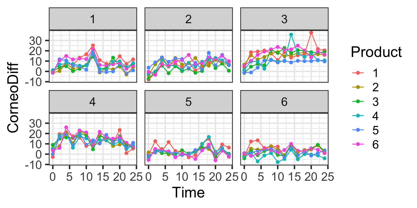
We could try just fitting a linear regression. What do you expect?
lm1 <- lm(CorneoDiff ~ Time + Product, data=hyd.sm)
summary(lm1)
Call:
lm(formula = CorneoDiff ~ Time + Product, data = hyd.sm)

Residuals:
    Min      1Q  Median      3Q     Max
-17.791  -5.349  -1.164   4.415  29.691

Coefficients:
            Estimate Std. Error t value Pr(>|t|)
(Intercept)  9.79072    0.87716  11.162  < 2e-16 ***
Time        -0.05726    0.02720  -2.105  0.03577 *
Product2    -1.90238    1.10665  -1.719  0.08623 .
Product3    -2.80079    1.10665  -2.531  0.01169 *
Product4    -2.98016    1.10665  -2.693  0.00732 **
Product5    -3.02659    1.10665  -2.735  0.00646 **
Product6    -0.43929    1.10665  -0.397  0.69157
---
Signif. codes:  0 '***' 0.001 '**' 0.01 '*' 0.05 '.' 0.1 ' ' 1

Residual standard error: 7.172 on 497 degrees of freedom
Multiple R-squared:  0.03701,   Adjusted R-squared:  0.02538
F-statistic: 3.183 on 6 and 497 DF, p-value: 0.004487gf_point(CorneoDiff ~ Time | Subjects, color=~Product, data=hyd.sm) |>
gf_line(CorneoDiff ~ Time | Subjects, color=~Product, data=hyd.sm) |>
gf_lims(x=c(0,24)) |>
gf_abline(intercept=7.86, slope=0.05608)
For the linear regression:
acf(resid(lm1))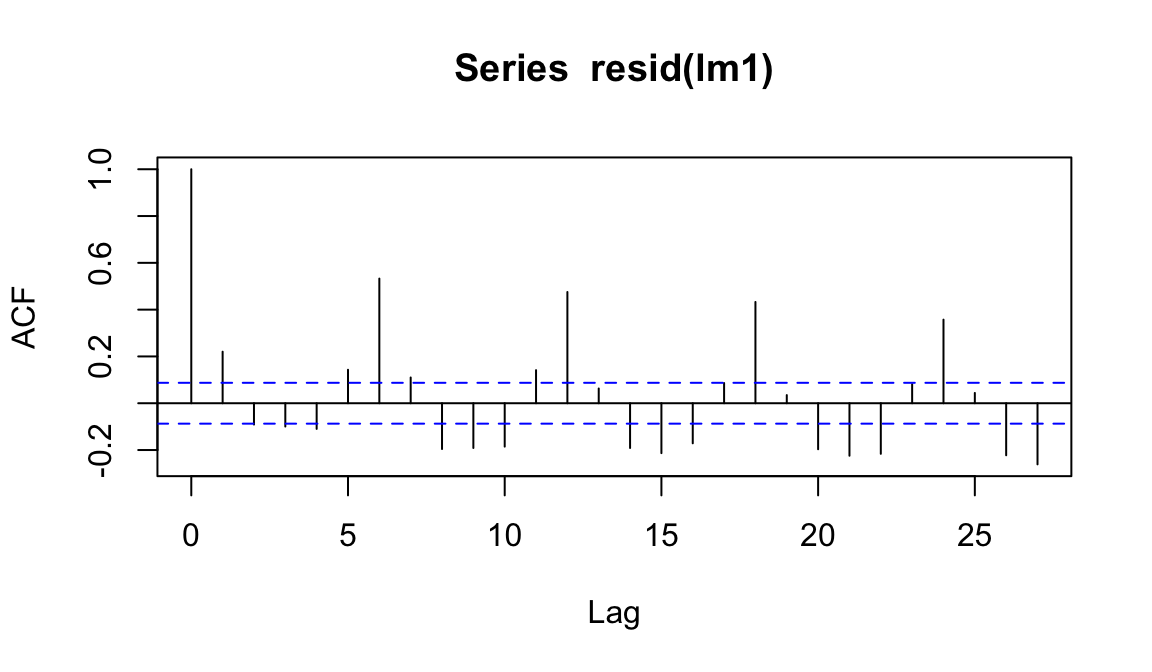
hyd.sm <- arrange(hyd.sm,Time, Subjects)
lm1 <- lm(CorneoDiff ~ Time + Product, data=hyd.sm)
acf(resid(lm1))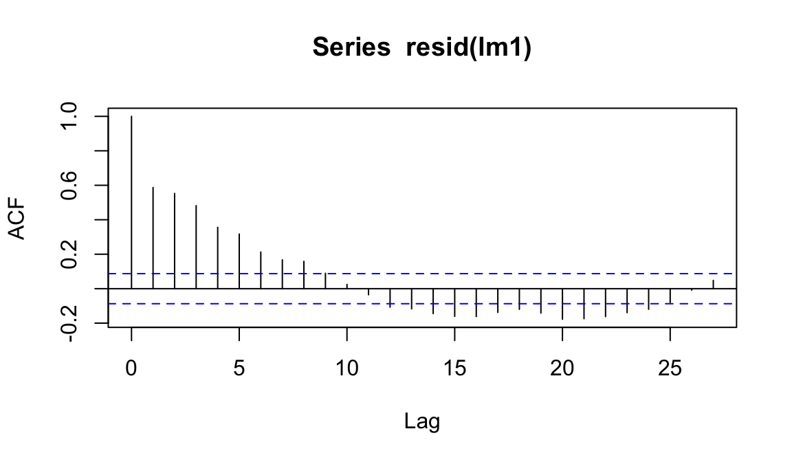
As we expected, things do not look good…
We tried a linear regression and encountered two problems:
A potential solution we will invesitgate today is to use a generalized estimating equation (GEE) instead of a GLM. GEEs:
What residual correlation structures can be accomodated in this framework?
corstr=independence’`)corstr=exchangeable’`)corstr=ar1’`)corstr=unstructured’`)library(geepack)
Attaching package: 'geepack'The following object is masked from 'package:MuMIn':
QIChyd <- arrange(hyd, Subjects, Time)
lm1 <- lm(CorneoDiff ~ Time + Product, data=hyd)
summary(lm1)
Call:
lm(formula = CorneoDiff ~ Time + Product, data = hyd)

Residuals:
     Min       1Q   Median       3Q      Max
-22.5776  -5.3165  -0.0275   5.1061  28.0872

Coefficients:
            Estimate Std. Error t value Pr(>|t|)
(Intercept) 11.42313    0.48032  23.782  < 2e-16 ***
Time        -0.09552    0.01489  -6.413 1.85e-10 ***
Product2    -2.08655    0.60598  -3.443 0.000589 ***
Product3    -2.49940    0.60598  -4.125 3.90e-05 ***
Product4    -1.96107    0.60598  -3.236 0.001235 **
Product5    -2.37238    0.60598  -3.915 9.41e-05 ***
Product6    -0.50833    0.60598  -0.839 0.401669
---
Signif. codes:  0 '***' 0.001 '**' 0.01 '*' 0.05 '.' 0.1 ' ' 1

Residual standard error: 7.17 on 1673 degrees of freedom
Multiple R-squared:  0.04082,   Adjusted R-squared:  0.03738
F-statistic: 11.87 on 6 and 1673 DF,  p-value: 4.489e-13
gee.ind <- geeglm(CorneoDiff ~ Time + Product, data=hyd,
id = Subjects, corstr='independence')
summary(gee.ind)
Call:
geeglm(formula = CorneoDiff ~ Time + Product, data = hyd, id = Subjects,
    corstr = "independence")

 Coefficients:
            Estimate  Std.err   Wald Pr(>|W|)
(Intercept) 11.42313  1.20102 90.462  < 2e-16 ***
Time        -0.09552  0.02342 16.638 4.52e-05 ***
Product2    -2.08655  0.98810  4.459   0.0347 *
Product3    -2.49940  1.03782  5.800   0.0160 *
Product4    -1.96107  1.02207  3.681   0.0550 .
Product5    -2.37238  1.32981  3.183   0.0744 .
Product6    -0.50833  0.95744  0.282   0.5955
---
Signif. codes:  0 '***' 0.001 '**' 0.01 '*' 0.05 '.' 0.1 ' ' 1

Correlation structure = independence
Estimated Scale Parameters:

            Estimate Std.err
(Intercept)     51.2   4.017
Number of clusters:   20  Maximum cluster size: 84
gee.ar1 <- geeglm(CorneoDiff ~ Time + Product, data=hyd,
id = Subjects, corstr='ar1')
summary(gee.ar1)
Call:
geeglm(formula = CorneoDiff ~ Time + Product, data = hyd, id = Subjects,
    corstr = "ar1")

 Coefficients:
            Estimate Std.err  Wald Pr(>|W|)
(Intercept)  11.4005  1.3968 66.61  3.3e-16 ***
Time         -0.2045  0.0322 40.27  2.2e-10 ***
Product2     -2.2329  0.9941  5.04   0.0247 *
Product3     -2.7965  1.0486  7.11   0.0077 **
Product4     -2.4137  1.0402  5.38   0.0203 *
Product5     -2.9857  1.3513  4.88   0.0271 *
Product6     -1.2880  0.9735  1.75   0.1858
---
Signif. codes:  0 '***' 0.001 '**' 0.01 '*' 0.05 '.' 0.1 ' ' 1

Correlation structure = ar1
Estimated Scale Parameters:

            Estimate Std.err
(Intercept)     56.9    4.48
  Link = identity

Estimated Correlation Parameters:
      Estimate Std.err
alpha    0.951 0.00905
Number of clusters:   20  Maximum cluster size: 84
gee.exch <- geeglm(CorneoDiff ~ Time + Product, data=hyd,
id = Subjects, corstr='exchangeable')What is the same (or similar) and what is very different between the models?
We can use a specific variance of QIC, \(QIC_{R}\), to compare models with different correlation structures:
library(MuMIn)
# QIC(gee.ind, gee.exch, gee.ar1, typeR=TRUE)
How can we interpret this result?
Model assessment for a GEE is mostly the same as for the corresponding linear regression or GLM (Poisson, Logistic, etc.)
We were using GEEs to try to correct for issues with non-independent residuals. How does the residual plot change for a GEE relative to the corresponding (g)lm? Does it change? Should it?
acf(resid(lm1), main='LM ACF')
acf(resid(gee.ind), main='GEE ACF')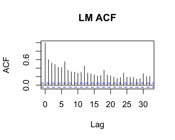
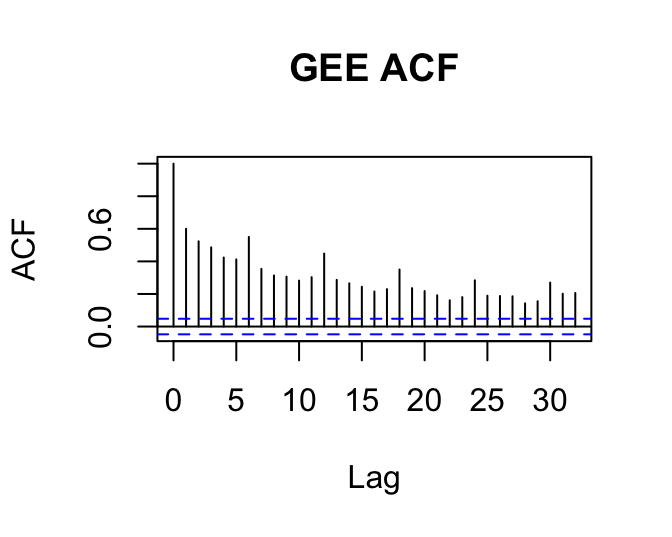
What is going on here?
We can use another variant of the QIC to do model selection to determine which variables are important to retain in a GEE model.
gee.ind <- update(gee.ind, na.action='na.fail')
dredge(gee.ind, rank='QIC', typeR=FALSE)
Fixed term is "(Intercept)"Global model call: geeglm(formula = CorneoDiff ~ Time + Product, data = hyd, na.action = "na.fail",
id = Subjects, corstr = "independence")
---
Model selection table
(Intrc) Prdct Time qLik QIC delta weight
1 8.46 -840 1729 0.00 0.954
3 9.85 -0.0955 -840 1735 6.06 0.046
2 10.03 + -840 1756 26.88 0.000
4 11.42 + -0.0955 -840 1763 33.71 0.000
Models ranked by QIC(x, typeR = FALSE) How would you interpret these results and present them to the cosmetics company that collected the data?
As for models we studied previously, we can make prediction plots to visualize the relationships a model specifies between the predictor and response variables.
However, we can not use predict() to get model predictions with standard errors from a GEE.
pred_plot() works, though; for example:
s245::pred_plot(gee.ind, 'Product') |>
  gf_labs(y = 'CorneoDiff')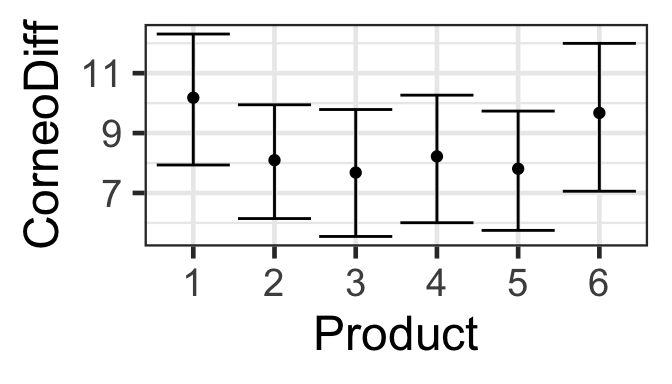
Once again we’re grateful for the parametric bootstrap! (This time, pred_plot() is silently doing the work for us.)