gf_dhistogram(~AN3, data=wt, binwidth=1) |>
  gf_labs(x='Weight (kg)', y='Probability\nDensity') |>
  gf_fitdistr(dist='dnorm', size=1.3) |>
  gf_refine(scale_x_continuous(breaks=seq(from=0, to=30, by=2)))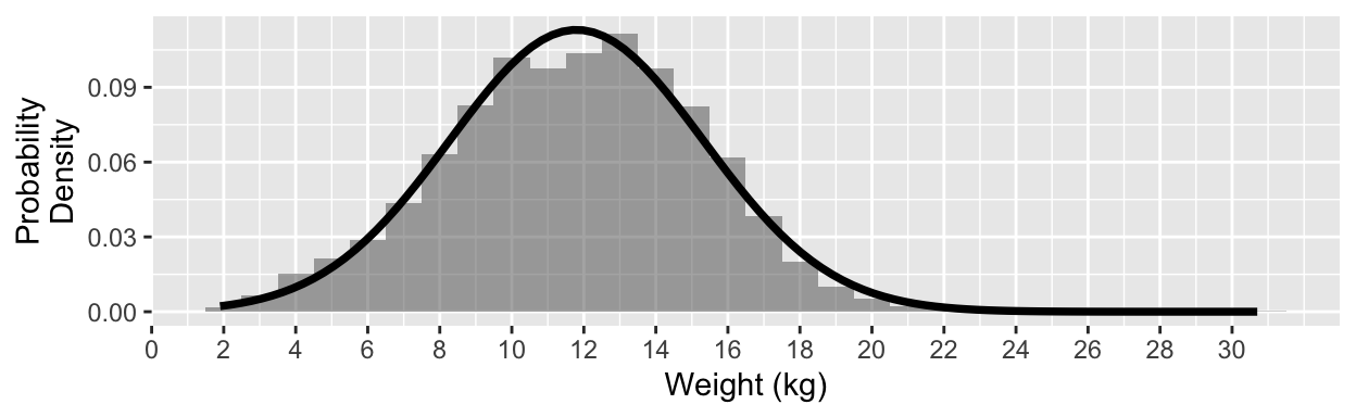
In the last section, we said that “likelihood” is a measure of goodness-of-fit of a model to a dataset. But what is it exactly and just how do we compute it?
Today’s dataset was collected in Senegal in 2015-2016 in a survey carried out by UNICEF, of 5440 households in the urban area of Dakar, Senegal. Among these households, information was collected about 4453 children under 5 years old, including their
gf_dhistogram(~AN3, data=wt, binwidth=1) |>
gf_labs(x='Weight (kg)', y='Probability\nDensity') |>
gf_fitdistr(dist='dnorm', size=1.3) |>
gf_refine(scale_x_continuous(breaks=seq(from=0, to=30, by=2)))
\[ f(x) = \frac{1}{\sqrt{2\pi\sigma^2}} e^{-\frac{(x-\mu)^2}{2\sigma^2}} \]
The distribution of weights looks quite unimodal and symmetric, so we will model it with a normal distribution with mean 11.8 and standard deviation 3.53 (N( \(\mu=\) 11.8, \(\sigma=\) 3.53), black line).
If you had to predict the weight of one child from this population, what weight would you guess?
Is it more likely for a child in Dakar to weigh 10kg, or 20kg? How much more likely?
What is the probability of a child in Dakar weighing 11.5 kg?
Which is more likely: three children who weigh 11, 8.2, and 13kg, or three who weigh 10, 12.5 and 15 kg?
How did you:
What did you have to assume about the set of observations?
What if we think of this situation as a linear regression problem (with no predictors)?
lm_version <- lm(AN3 ~ 1, data = wt)
summary(lm_version)
Call:
lm(formula = AN3 ~ 1, data = wt)

Residuals:
    Min      1Q  Median      3Q     Max
-9.8964 -2.3964  0.1036  2.4036 18.9036

Coefficients:
            Estimate Std. Error t value Pr(>|t|)
(Intercept) 11.79644    0.05435   217.1   <2e-16 ***
---
Signif. codes:  0 '***' 0.001 '**' 0.01 '*' 0.05 '.' 0.1 ' ' 1

Residual standard error: 3.529 on 4216 degrees of freedom
  (235 observations deleted due to missingness)
Finally, now, we can understand what we were computing when we did
logLik(lm_version)'log Lik.' -11301.19 (df=2)For our chosen regression model, we know that the residuals should have a normal distribution with mean 0 and standard deviation \(\sigma\) (estimated Residual Standard Error from R summary() output).
For each data point in the dataset, for a given regression model, we can compute a model prediction.
We can subtract the prediction from the observed response-variable values to get the residuals.
We can compute the likelihood (\(L\)) of this set of residuals by finding the likelihood of each individual residual \(e_i\) in a \(N(0, \sigma)\) distribution.
To get the likelihood of the full dataset given the model, we use the fact that the residuals are independent (they better be, because that was one of the conditions of of linear regression model) – we can multiply the likelihoods of all the individual residuals together to get the joint likelihood of the full set.
That is the “likelihood” that is used in the AIC and BIC calculations we considered earlier.