Chapter 13 Non-constant variance (and other unresolved problems)

So far, we have worked to assemble a tool-kit that allows us to fit appropriate regression models for a variety of types of response and predictor variables. If we fit an appropriate model (conditions are met) to an appropriate dataset (representative sample of the population of interest), we should be able to draw valid conclusions – but as we have seen, if conditions are not met, then our conclusions (model predictions, judgements about which predictors are important, etc.) may all be unreliable.

So what can we do if we’ve fit the best model we know how to fit, and it’s still not quite right? We have seen a number of examples so far where, even after we fit a model with what seem to be the right family and sensible predictors, conditions are not met. The most common problems are non-constant variance of residuals (often seen with non-normal residuals), and non-independent residuals. Solutions for non-independent residuals are coming soon, in future sections. Here we’ll review options (some already in our tool-kit, and some new) to try to improve the situation when non-constant variance (NCV) is present.

What can we try if a model seems to fit data well, except for the fact that the constant variance condition doesn’t hold (for linear regression) or the mean-variance relationship is not as expected (GLMs etc.)? (Note: this problem is also often accompanied by right skew in the distribution of the residuals.) Possible solutions are presented approximately in order of desirability…

13.0.1 Already in Our Tool Box: Make sure the model is “right”

Improving the model specification sometimes corrects a problem with non-constant variance. Make sure you have considered:

Is the right “family” being used for the data type being modelled?
Are all the variables that you think are important predictors (and are available to you in the data) included in the model?

13.0.2 Already in Our Tool Box: Models that estimate dispersion parameters

Negative binomial (and quasi-Poisson) models include estimation of a dispersion parameter that helps to account for over- or under-disperion (that is - the variance is larger, or smaller, than the mean value). If one of these models is being used (or is appropriate for the data) - NCV should be accounted for! (We can also verify this: If all is working well, the Pearson residuals will have constant variance.)

13.0.3 Gamma GLMs

If you are fitting a linear regression and:

The response variable of interest is non-negative, and
There is right skew in residuals and/or
There is non-constant variance of residuals…

You may want to try fitting a model using the Gamma family (link = 'log' or link = 'inverse' link functions are the most common). If needed you can use model assessment plots and/or model selection criteria (AIC, BIC…) to decide between link functions. For example:

gamma.mod <- glm(resp ~ pred1 + pred2, data=dataset,
                 family=Gamma(link='log')) # or can use link='inverse'

13.0.4 Beta GLMs

If your response variable happens to be bounded between 0-1 (but NOT a probability, so that a binary data regression would not be appropriate), you can also try a Beta regression (using the beta distribution). Since the shape of the distribution is extremely flexible, it will help with residuals whose distribution is not as expected. The variance of the beta distribution also does depend on its mean, so it is likely to be better than a linear model at addressing NCV. A code example is below. You must use glmmTMB() to fit this model.

beta_model <- glmmTMB(response ~ predictor1 + predictor2,
                      data=my_data,
                      family=beta_family(link='logit'))

13.0.5 Transformations

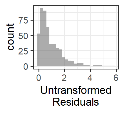
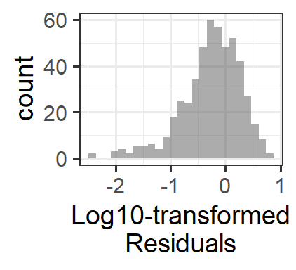
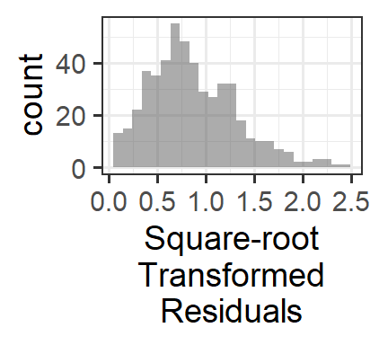
In some cases, a logarithmic or square-root transformation of the response variable can correct a problem with the variance of the residuals. This is most sensible as a solution if the log(variable) or sqrt(variable) makes some “sense” to a human…for example, if the response variable is wages in dollars, then log10(wages) is kind of the order of magnitude of the salary, which makes some sense as a measure of income. Another example: sound pressure is measured in \(\mu Pa\), but we perceive sound logarithmically, so that a sound that has 10 times greater pressure “sounds” about twice as loud. So log10(sound_pressure) could be a sensible metric.

Why does this work? These transformations don’t affect the magnitude of small residual values very much, but they make large residuals get a lot smaller. The result is that the histogram of residuals has less right skew and the large-magnitude residuals (the ones causing the “flare” of the “trumpet” in the residuals vs. fitted plot) get much smaller.

13.0.6 Modelling non-constant variance

If your model is a linear regression, then there are a few specialized fitting functions that can allow you to fit models with non-constant variance of the residuals.

For multiple linear regression (original fit with lm()), you can use gls() from package nlme and add input weights=varPower() – inputs are otherwise the same as for lm().

require(nlme)
nls(response ~ pred1 + pred2, data=dataset,
    weights=varPower())

If you’re interested in learning more about this method (and other options for specification of the form of the non-constant variance), see the references below in R (you will not be held responsible for the information contained in these help files for STAT 245 - just provided for further reference.)

?nlme::nls
?nlme::varClasses